Sigma Delta without Math – Part 2 – 2021-12-04
Last time around I talked about strategies for halftoning graphics, and made the key point that “noise” and “objectionable noise” are not the same thing.
I haven’t yet mentioned, though, the class of dither patterns which has been used most commonly since the advent of the desktop printer – namely Error Diffusion.
The most well-known of these is Floyd-Steinberg dithering. Once again, the principle is to modulate the source data in some way before applying the threshold function – but instead of using some external source of modulation (such as a dither matrix or a random number), we use the error from previous pixels instead. So, for example, if we have a pixel of intensity 0.7, we would apply the threshold function giving us a pixel of intensity 1. The difference between what we wanted and what we got is -0.3, so we add that to the next pixel value before applying the threshold function, each time feeding the error forward to subsequent pixels.
(Since dithering graphics is generally done in two dimensions, scanline by scanline, the error is typically split and distributed to the four neighbouring pixels which haven’t yet been processed.)
The result will no doubt look familiar to anyone who’s ever printed something on an inkjet printer:
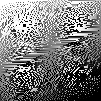
And if we compare this with the original, to see the error:
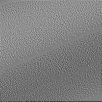
Now that’s quite impressive. From any significant distance away this looks smooth, thanks to the low-pass filtering effect of human vision when individual features are too small to see. (It’s also perceived as being close to mid-grey – i.e. zero-error – all over, even though it isn’t. There’s some variation due to the fact that I haven’t taken gamma into account when creating these illustrations – that’s a story for another day!)
This class of dithering algorithm is extremely good at making sure the bulk of the error is high-frequency, and thus invisible from a distance. This effect is called noise shaping – it exploits the principle we explored last time that “noise” and “objectionable noise” are not the same thing; doing it effectively – both in one and two dimensions – has been the subject of much research over the years.
If you’re thinking “Aha! We could use exactly the same principles in one dimension rather than two when processing audio”, then congratulations – you’ve just invented Sigma Delta modulation. Just like with Floyd-Steinberg dithering, the idea is to feed the quantisation error forward into the next sample, which has the effect of letting only the highest frequency components of the error through into the output.
So lets take a look at how we can apply these principles to an audio signal:
Since we’ve examined several different classes of graphical dithering algorithm, let’s do the same with an audio signal. To avoid angering the copyright gods I’ll use a brief audio snippet here which I recorded some time ago, shortly after attacking a cheap Lidl nylon guitar with a Dremel, and installing an undersaddle pickup!
All the DACs I demonstrate here will have a common interface, so they’re interchangeable. Here’s the interface – in the interests of brevity I’ll only show it the once:
module <name>_dac #(parameter signalwidth=16)
(
   input clk,
   input reset_n,
   input [signalwidth-1:0] d,
   output q
);
reg q_reg;
assign q=q_reg;
So following this boilerplate, we can try out various DAC strategies. Firstly, let’s create the equivalent of the simple threshold function that we started with last time:
always @(posedge clk or negedge reset_n) begin
   if(!reset_n) begin
      q_reg <= 1'b0;
   end else begin
      q_reg <= d[signalwidth-1];
   end
end
So what we’re doing here is outputting a 1 when the topmost bit of the input signal is a 1, i.e. when the input signal is in the top half of its range. As you might imagine, this doesn’t sound great: (To protect your eardrums I’ve massively reduced the volume of this sample!)
I mean, you might actually *like* how it sounds – but it can’t be called a faithful reproduction. (It’s probably a more faithful reproduction of how the guitar sounded while I was wielding the Dremel…)
So next we added random noise followed by a threshold function – let’s do the same with audio. To do this I’m going to use a linear feedback shift register – I’m not going to include full source here, but it’s all present in the github repo which I’ll link to later.
wire [31:0] noise;
lfsr #(.width(32)) mylfsr
(
    .clk(clk),
    .reset_n(reset_n),
    .e(1'b1),
    .save(1'b0),
    .restore(1'b0),
    .q(noise)
);
reg [signalwidth:0] sigma;
always @(posedge clk or negedge reset_n) begin
   if(!reset_n) begin
      q_reg <= 1'b0;
   end else begin
      sigma<=noise[signalwidth-1:0]+d;
      q_reg <= sigma[signalwidth];
   end
end
What I’m doing here is creating a 32-bit LFSR, so that the noise doesn’t repeat too quickly. I’m adding the lower 16 bits to the incoming audio signal (yes, I know, that’s not the correct way to use an LFSR), and outputting a 1 if the sum overflows into a 17th bit.
So how does this sound?
Well, OK, still awful – but the recording’s clearly much more intelligible, behind the noise. It would be interesting to run the noise through a high-pass filter to make it less audible, and see if it was still as effective at revealing the recording.
So next we looked at a traditional litho printing dot screen – where the spacing of the dots was fixed, with their size being determined by the underlying signal. Let’s try the same in one dimension – which would be Pulse Width Modulation.
This can be conceptualised as adding a sawtooth wave to the signal, then outputting a 1 when the result overflows – but it’s simpler to express as a comparison with the sawtooth wave (a simple free-running counter) – and looks like this:
reg [pwmwidth-1:0] pwmcounter;
always @(posedge clk or negedge reset_n) begin
   if(!reset_n) begin
      q_reg <= 1'b0;
      pwmcounter<={pwmwidth{1'b0}};
   end else begin
      pwmcounter<=pwmcounter+1'b1;
      if(pwmcounter > d[signalwidth-1:signalwidth-pwmwidth])
         q_reg<=1'b0;
      else
         q_reg<=1'b1;
   end
end
This actually sounds pretty good! The downside of this method is that the resolution is limited – the more bits we give to our counter (pwmwidth) the more resolution we have in the output – however if the counter has enough bits that its period strays down into the audible spectrum then we’ll hear a constant whine overlaid with the audio. If the period’s short enough for the whine to be above the limit of human hearing, then we’re likely to have a crunchy low-bit-depth sound. Notice particularly that there’s some crunchy background noise in the quieter parts.
Now let’s consider a version which feeds error forward to the next sample, similar to the Floyd Steinberg graphical halftone I showed at the start of this article.
What I’ll do here is add each incoming sample to an accumulator – any time this accumulator overflows into a 17th bit we will output a 1, and whether or not it overflowed the remaining 16 bits will be our error term for the next sample.
reg [signalwidth:0] sigma;
 always @(posedge clk or negedge reset_n) begin
    if(!reset_n) begin
       sigma <= {1'b1,{signalwidth{1'b0}}};
       q_reg <= 1'b0;
    end else begin
       sigma <= sigma[signalwidth-1:0] + d;
       q_reg <= sigma[signalwidth];
    end
 end
Interestingly this is simpler than everything that’s come before except the threshold DAC. Does it sound good, though?
Well it’s clearly the best result so far, however there’s an odd effect in the quiet bit at the end of the recording. Simple (i.e. 1st order) Sigma Delta DACs suffer from the same problem as PWMs in that they need to run at an unreasonably high frequency in order to keep the noise beyond the range of human hearing. To solve this, we would have to explore the realms of 2nd- and higher order DACs – basically the same principle but with more complicated feedback structures, to shift the noise into the higher frequencies more efficiently – and that, unfortunately, is where we fall into a quagmire of heavy maths and deep magic!
Nonetheless, using a largely intuitive process I was able to create a 2nd order DAC capable of this result:
I’ll talk about it in more depth next time.
For now, though, the verilator-based testbenches which created these recordings can be found at https://github.com/robinsonb5/DACTests